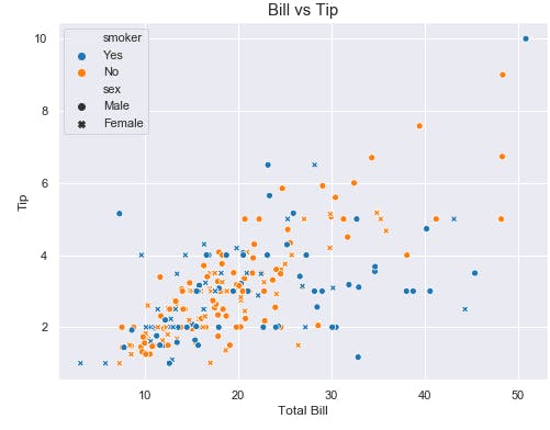
Scatter plots are great for visualizing relationships between two quantitative variables. The data is represented as points scattered over the plot axes. It shows a trend or pattern in data as can be seen below

A common issue faced with scatter plots is the issue of Overplotting.

Overplotting happens when there are too many overlapping points as a result of a large sample size or discrete variables. The plot forms a kind of blob that makes it difficult to understand the pattern in the data.

Check out this plot from a dataset on various car attributes.

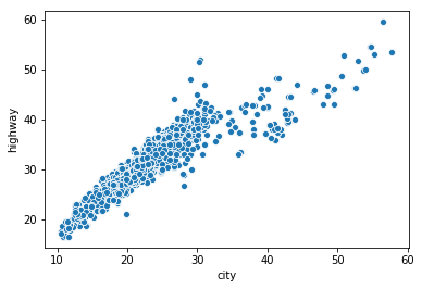
The scatterplot shows relationship between fuel mileage ratings for city vs. highway driving

The plot does show a linear trend, however, there's a big blob of data points at the bottom left that makes it difficult to see what exactly is going on there. This is overplotting. And i'll be talikng about three ways we can solve this issue.

1. Sampling: Here, a smaller portion of the dataset is plotted to see the actual effect which is obscured by the overlapping points. The sampling is done randomly to make sure it is a true representative of the whole population.

Here's the scatterplot of a random sample(df_samp) of the same dataset(df) from above after.

df_samp = df.sample(frac = .01, random_state = 23)
sns.scatterplot(data = df_samp, x = "city", y = "highway");

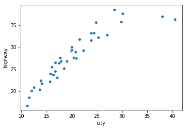
As you can see, its easier to see the relationship between the city and highway ratings

2. Transparency: This invlves changing the appearance of data points to see those that are stacked on top of one another more clearly. A dark area indicates that the data points are overlapping. This can be achieved by adding an alpha value between 0 and 1.

sns.scatterplot(data = df, x = "city", y = "highway", alpha = 0.2);

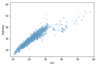
The darker areas clearly show that most of ratings for city fall between 10 and 30 and most of the ratings for highway fall between 20 and 40. Also, for the lower part of plot, the highway ratings are generally more than the city rating, then the trnd seems to get more uniform towards the middle and for the upper art of the plot, it can be seen that some of the ratings for city were more than those for the highway fuel mileage.

That's what transparency can do! This can be very useful when dealing with discrete variables.

3. Jittering No, it's not the kind you get when you're nervous. Jittering in this context, means changing the x and/or y location of data points slightly to add some noise. This is especially used for discrete variables and it widens the distribution at each point so that it is easier to see. Note: for small datasets, a swarm plot is a much better alternative to jittering.

Check out this article for more details on jittering.

Sometimes, your dataset could be too large for transparency to make sense or it could be a plot of two discrete discrete variables, then a heat map would be a better option.

You can also treat the discrete variables as categorical variables and use a violin plot instead.

What other method would you use in the case of overplotting? Let us know in the comments.